Finite Difference Method

This document uses the open source Jupyter Notebook and the Python programming language to demonstrate a finite difference numerical method for solving a differential equation.

%matplotlib inline

# Required libraries
import numpy as np
import matplotlib.pyplot as plt
import seaborn as sns

# Seaborn aesthetics
sns.set_context("paper", font_scale=1.8,
    rc={"lines.linewidth": 3, "figure.figsize": (10,6)})
sns.set_style("ticks")

Beam Deflection Problem

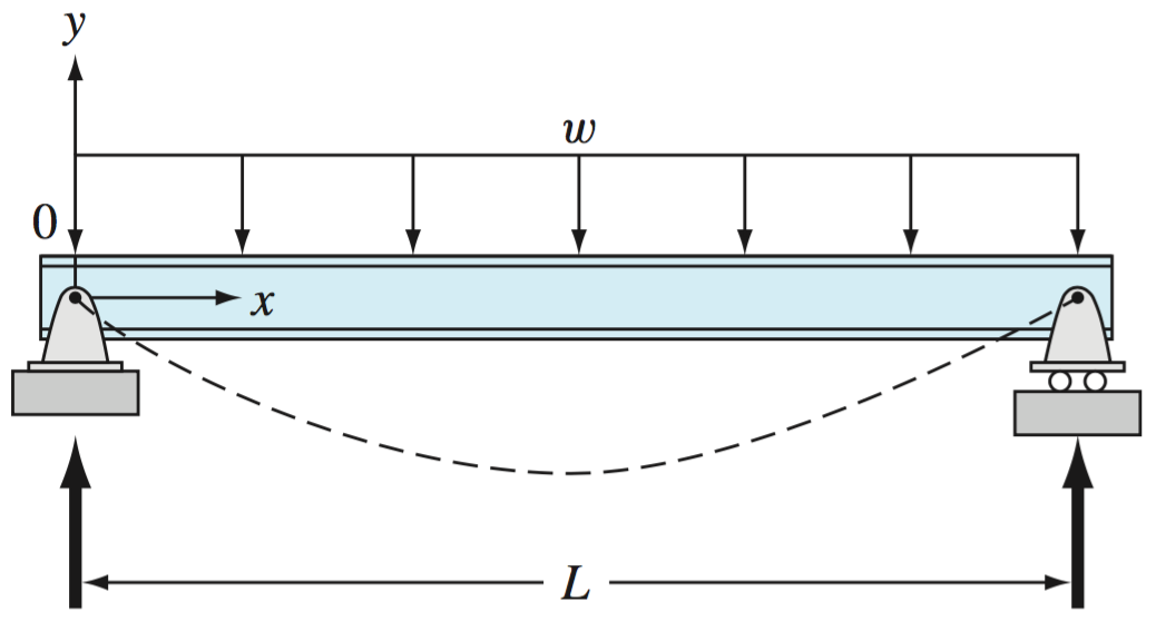Figure 1. Uniformly-loaded beam (Chapra, p. 639).

The basic differential equation of the elastic curve for a simply supported, uniformly loaded beam (Fig. 1) is given as

\begin{equation} EI \frac{d^2y}{dx^2} = \frac{wLx}{2} - \frac{wx^2}{2} \tag{3} \end{equation}

where $E=$ the modulus of elasticity, and $I=$ the moment of inertia. The boundary conditions are $y(0)=y(L)=0$. Solve for the deflection of the beam using the finite-difference approach $(\Delta x = 0.6 m)$. The following parameter values apply: $E = 200$ GPa, $I = 30,000$ cm$^4$, $w = 15$ kN/m, and $L = 3$ m. Compare your numerical results to the analytical solution:

\begin{equation} y = \frac{wLx^3}{12EI} - \frac{wx^4}{24EI} - \frac{wL^3x}{24EI} \tag{4} \end{equation}

Analytical Solution

def y(x):
"""
Vertical deflection, y, of the beam in 10E-5 m.
"""
E = 200 _ 10**9 # Pa
I = 30000 / 100**4 # m^4
w = 15 _ 1000 # N/m
L = 3 # m
return ((w*L*x**3)/(12*E*I) - (w\*x**4)/(24*E*I) - \
 (w*x*L**3)/(24*E*I)) \* 10**5

Central Difference Method

def cdiff_beam(L,ya,yb,n):
    """
    Approximate vertical deflection, y, of the beam in 10E-5 m,
    using central difference method.
    Args:
    L = length of the beam, m
    ya = vertical deflection at x = 0
    yb = vertical deflection at x = L
    n = desired number of interior segments

    """
    E = 200 _ 10**9 # Pa
    I = 30000 / 100**4 # m^4
    w = 15 _ 1000 # N/m
    i = 0
    x = 0
    dx = L/n
    X = [x]
    A = np.zeros(shape=(n+1,n+1))
    b = np.zeros(shape=(n+1,1))

    while i < n-1:
        i = i + 1
        x = x + dx
        b[i] = dx**2 * (1/(2*E*I)) * (w*L*x - w\*x**2)
        A[i][i] = -2
    if i < n:
        A[i][i+1] = 1
        A[i][i-1] = 1
    X = np.append(X, x)
    A[0][0] = 1
    A[n][n] = 1
    b[0] = ya
    b[n] = yb

    X = np.append(X, x+dx)
    Y = np.linalg.solve(A,b)
    # print(A); print(b)
    return X, Y

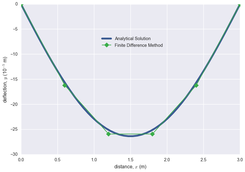
Plot of Solutions

x = np.linspace(0,3)
X,Y = cdiff_beam(3,0,0,8)

plt.plot(x,y(x), lw=7, alpha=0.6, label="Analytical Solution")
plt.plot(X,Y*10**5, "o-", lw=2, ms=8, color="#c44e52", label="Finite Difference Method")
plt.legend(bbox_to_anchor=[0.665, 0.81])
plt.xlabel("distance, $x$ (m)")
plt.ylabel("deflection, $y$ (10$^{-5}$ m)")
sns.despine()
plt.show()

Loaded Beam